42 how to change excel chart data labels to custom values

How to add or move data labels in Excel chart? In Excel 2013 or 2016. 1. Click the chart to show the Chart Elements button . 2. Then click the Chart Elements, and check Data Labels, then you can click the arrow to choose an option about the data labels in the sub menu. See screenshot: In Excel 2010 or 2007. 1. click on the chart to show the Layout tab in the Chart Tools group. See ... Create Dynamic Chart Data Labels with Slicers - Excel Campus The next step is to change the data labels so they display the values in the cells that contain our CHOOSE formulas. As I mentioned before, we can use the "Value from Cells" feature in Excel 2013 or 2016 to make this easier. You basically need to select a label series, then press the Value from Cells button in the Format Data Labels menu.

How to Customize Your Excel Pivot Chart Data Labels - dummies If you want to label data markers with a category name, select the Category Name check box. To label the data markers with the underlying value, select the Value check box. In Excel 2007 and Excel 2010, the Data Labels command appears on the Layout tab. Also, the More Data Labels Options command displays a dialog box rather than a pane.

How to change excel chart data labels to custom values

Change the format of data labels in a chart To get there, after adding your data labels, select the data label to format, and then click Chart Elements > Data Labels > More Options. To go to the appropriate area, click one of the four icons ( Fill & Line, Effects, Size & Properties ( Layout & Properties in Outlook or Word), or Label Options) shown here. › color-chart-bars-by-valueHow to color chart bars based on their values - Get Digital Help May 11, 2021 · Column chart. Advanced charts. Custom data labels(1) Custom data labels(2) Label line chart series. Between tick marks. Add line to chart. Add pictures to chart axis. Color chart bars based on their values. Primary data hidden. Stock chart with 2 series. Adjust axis value range. Color based on prior val. Hide specific columns. Dynamic stock ... Datalabels formatter - animadigomma.it ShowValue ), the series name ( DataLabelBase First add data labels to the chart (Layout Ribbon > Data Labels) Define the new data label values in a bunch of cells, like this: Now, click on any data label. properties and restart the server: com. jaspersoft. md doc table datalabels 플러그인을 세팅하면 그래프 안에 수치가 주욱 ...

How to change excel chart data labels to custom values. Custom Chart Data Labels In Excel With Formulas Follow the steps below to create the custom data labels. Select the chart label you want to change. In the formula-bar hit = (equals), select the cell reference containing your chart label's data. In this case, the first label is in cell E2. Finally, repeat for all your chart laebls. excel - How do I update the data label of a chart? - Stack ... If the chart is actually using the value which changed (from 95 to 90), then the label should reflect that change automatically. There are some exceptions to this maybe, but without being able to see/know how your data and chart are configured, it's tough to speculate on why your chart isn't behaving the "normal" way. peltiertech.com › make-a-copied-chart-link-to-new-dataMake a Copied Chart Link to New Data - Peltier Tech Mar 30, 2009 · The references in the chart did not change, so the pasted chart still referenced the original data. Instead of copying just the chart, this time copy the sheet with its chart. The new sheet is now named ‘Sheet1 (2)’, meaning copy 2 of Sheet1, and we see from the highlighted range and series formula that the chart on the new sheet references ... Custom Data Labels with Colors and Symbols in Excel Charts ... To apply custom format on data labels inside charts via custom number formatting, the data labels must be based on values. You have several options like series name, value from cells, category name. But it has to be values otherwise colors won't appear. Symbols issue is quite beyond me.

Using the CONCAT function to create custom data labels for ... Use the chart skittle (the "+" sign to the right of the chart) to select Data Labels and select More Options to display the Data Labels task pane. Check the Value From Cells checkbox and select the cells containing the custom labels, cells C5 to C16 in this example. It is important to select the entire range because the label can move based ... support.microsoft.com › en-us › officeEdit titles or data labels in a chart - support.microsoft.com Change the position of data labels. You can change the position of a single data label by dragging it. You can also place data labels in a standard position relative to their data markers. Depending on the chart type, you can choose from a variety of positioning options. On a chart, do one of the following: editing Excel histogram chart horizontal labels ... On the one hand, since you have found the workaround, we'd suggest you use the workaround. On the other hand, if you want to use such chart, you can also create bar chart. However, you may need to calculate the number of those data, then you can insert bar chat. And it will show the effect you want. blogs.library.duke.edu › data › 2012/11/12Adding Colored Regions to Excel Charts - Duke Libraries ... Nov 12, 2012 · Change the “years… in decline” series to an area chart; Select and adjust the x axis labels and ticks; Adjust the y axis range; Customize the color, label, and order of the data series; The basic mechanism of the colored regions on the chart is to use Excel’s “area chart” to create rectangular areas.

Custom data labels in a chart - Get Digital Help Press with right mouse button on on any data series displayed in the chart. Press with mouse on "Add Data Labels". Press with mouse on Add Data Labels". Double press with left mouse button on any data label to expand the "Format Data Series" pane. Enable checkbox "Value from cells". Improve your X Y Scatter Chart with custom data labels Press with right mouse button on on a chart dot and press with left mouse button on on "Add Data Labels" Press with right mouse button on on any dot again and press with left mouse button on "Format Data Labels" A new window appears to the right, deselect X and Y Value. Enable "Value from cells" Select cell range D3:D11 Use custom formats in an Excel chart's axis and data labels Use custom formats in an Excel chart's axis and data labels . Adding a custom format to a chart's axis and data labels can quickly turn ordinary data into information. Excel Custom Chart Labels - My Online Training Hub Step 5: Replace the default labels with your custom labels: right-click the labels > Format Data Labels: From the 'Label Contains' list choose 'Category Name': Step 6: hide the Max series columns by formatting them with 'No fill': double-click the Max columns in the chart to open the 'Format Data Point' dialog box and under the ...

Excel - Butterfly Chart

How to add data labels from different column in an Excel ... Click any data label to select all data labels, and then click the specified data label to select it only in the chart. 3. Go to the formula bar, type =, select the corresponding cell in the different column, and press the Enter key. See screenshot: 4. Repeat the above 2 - 3 steps to add data labels from the different column for other data points.

[R-bloggers] Web Scraping with rvest + Astro Throwback (and 6 more aRticles)

Change axis labels in a chart - support.microsoft.com Right-click the category labels you want to change, and click Select Data. In the Horizontal (Category) Axis Labels box, click Edit. In the Axis label range box, enter the labels you want to use, separated by commas. For example, type Quarter 1,Quarter 2,Quarter 3,Quarter 4. Change the format of text and numbers in labels

charts - How do I create custom axes in Excel? - Super User

Custom Excel Chart Label Positions - My Online Training Hub Custom Excel Chart Label Positions - Setup. The source data table has an extra column for the 'Label' which calculates the maximum of the Actual and Target: The formatting of the Label series is set to 'No fill' and 'No line' making it invisible in the chart, hence the name 'ghost series': The Label Series uses the 'Value ...

How to Make a Pie Chart in Excel & Add Rich Data Labels to The Chart!

How to format axis labels as thousands/millions in Excel? 1. Right click at the axis you want to format its labels as thousands/millions, select Format Axis in the context menu. 2. In the Format Axis dialog/pane, click Number tab, then in the Category list box, select Custom, and type [>999999] #,,"M";#,"K" into Format Code text box, and click Add button to add it to Type list. See screenshot: 3.

Excel Vba Position Axis Tick Marks - excel chart vertical axis text labels u2022 my online ...

Excel Chart Data Labels-Modifying Orientation - Microsoft ... You can right click on the data label part then select Format Axis. Click on the Size & Properties tab then adjust the Text Direction or Custom Angle. Thanks, Mike Report abuse 6 people found this reply helpful · Was this reply helpful? Replies (7)

Custom data labels in a chart

Change the format of data labels in a chart To get there, after adding your data labels, select the data label to format, and then click Chart Elements > Data Labels > More Options. To go to the appropriate area, click one of the four icons ( Fill & Line, Effects, Size & Properties ( Layout & Properties in Outlook or Word), or Label Options) shown here.

31 How To Label Data Points In Excel

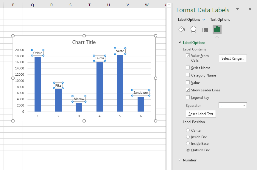
How to create Custom Data Labels in Excel Charts Two ways to do it. Click on the Plus sign next to the chart and choose the Data Labels option. We do NOT want the data to be shown. To customize it, click on the arrow next to Data Labels and choose More Options … Unselect the Value option and select the Value from Cells option. Choose the third column (without the heading) as the range.

How to Change Excel Chart Data Labels to Custom Values?

How to Change Excel Chart Data Labels to Custom Values? First add data labels to the chart (Layout Ribbon > Data Labels) Define the new data label values in a bunch of cells, like this: Now, click on any data label. This will select "all" data labels. Now click once again. At this point excel will select only one data label.

Share :