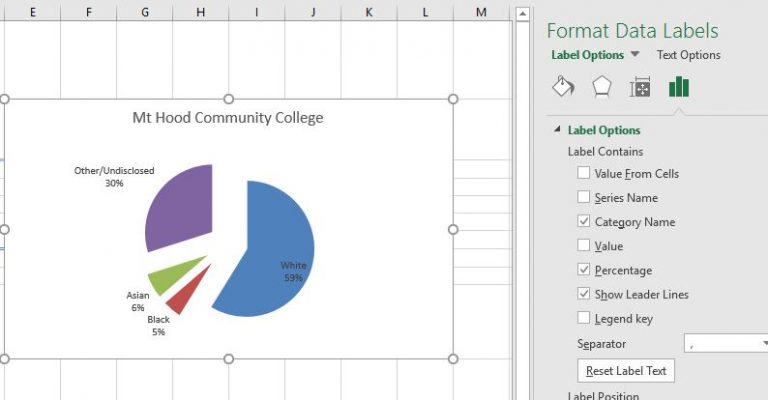
39 how to add percentage and category name data labels in excel

Add a DATA LABEL to ONE POINT on a chart in Excel All the data points will be highlighted. Click again on the single point that you want to add a data label to. Right-click and select ' Add data label '. This is the key step! Right-click again on the data point itself (not the label) and select ' Format data label '. You can now configure the label as required — select the content of ... How to Add Data Labels to an Excel 2010 Chart - dummies On the Chart Tools Layout tab, click Data Labels→More Data Label Options. The Format Data Labels dialog box appears. You can use the options on the Label Options, Number, Fill, Border Color, Border Styles, Shadow, Glow and Soft Edges, 3-D Format, and Alignment tabs to customize the appearance and position of the data labels.

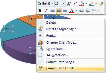
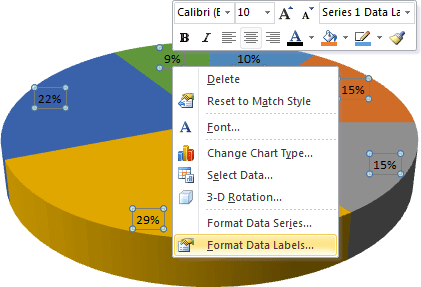
How to Add Percentage Axis to Chart in Excel To do this, we will select the whole table again, and then go to Insert >> Charts >> 2-D Columns: To show percentages on a second axis, we first need to click anywhere on the orange bars that we have on our graph (this is not easy in this example as they are rather small). Once we do, we will right-click on it, and then select Format Data Series:

How to add percentage and category name data labels in excel

Count and Percentage in a Column Chart - ListenData Download the workbook. Steps to show Values and Percentage. 1. Select values placed in range B3:C6 and Insert a 2D Clustered Column Chart (Go to Insert Tab >> Column >> 2D Clustered Column Chart). See the image below. Insert 2D Clustered Column Chart. 2. In cell E3, type =C3*1.15 and paste the formula down till E6. Adding data labels to a pie chart - Excel General - OzGrid Re: Adding data labels to a pie chart. Thanks again, norie. Really appreciate the help. I tried recording a macro while doing it manually (before my first post). But it didn't record anything about labels, much less making them bold. Excel charts: add title, customize chart axis, legend and data labels ... To add a label to one data point, click that data point after selecting the series. Click the Chart Elements button, and select the Data Labels option. For example, this is how we can add labels to one of the data series in our Excel chart: For specific chart types, such as pie chart, you can also choose the labels location.

How to add percentage and category name data labels in excel. Change the format of data labels in a chart To get there, after adding your data labels, select the data label to format, and then click Chart Elements > Data Labels > More Options. To go to the appropriate area, click one of the four icons ( Fill & Line, Effects, Size & Properties ( Layout & Properties in Outlook or Word), or Label Options) shown here. How to show data labels in PowerPoint and place them ... - think-cell To reset a label and (re-)insert text fields, use the label content control (Label content) or simply click on the exclamation mark, if there is one. Note: Due to a limitation in Excel only the first 255 characters of text in a datasheet cell will be displayed in a label in PowerPoint. Solved: change data label to percentage - Power BI pick your column in the Right pane, go to Column tools Ribbon and press Percentage button do not hesitate to give a kudo to useful posts and mark solutions as solution LinkedIn Message 2 of 7 1,613 Views 1 Reply MARCreading Regular Visitor In response to az38 06-09-2020 09:03 AM Hi @az38, Thanks for your help! How to Customize Your Excel Pivot Chart Data Labels - dummies To remove the labels, select the None command. If you want to specify what Excel should use for the data label, choose the More Data Labels Options command from the Data Labels menu. Excel displays the Format Data Labels pane. Check the box that corresponds to the bit of pivot table or Excel table information that you want to use as the label.

Pivot Chart Data Label Help Needed - Microsoft Community Open the Excel file with Pivot Chart and enabled with Data Labels> Click on the Labels displayed in the Chart> Right-click> Click Format Data Labels> Label Options> Number> In the Category, select the format as per your requirement. Here is the reference article: Change the format of data labels in a chart. Custom Chart Data Labels In Excel With Formulas Follow the steps below to create the custom data labels. Select the chart label you want to change. In the formula-bar hit = (equals), select the cell reference containing your chart label's data. In this case, the first label is in cell E2. Finally, repeat for all your chart laebls. Excel tutorial: How to use data labels When you check the box, you'll see data labels appear in the chart. If you have more than one data series, you can select a series first, then turn on data labels for that series only. You can even select a single bar, and show just one data label. In a bar or column chart, data labels will first appear outside the bar end. How to use Excel Data Model & Relationships - Chandoo.org Jul 01, 2013 · Handling large volumes of data in Excel—Since Excel 2013, the “Data Model” feature in Excel has provided support for larger volumes of data than the 1M row limit per worksheet. Data Model also embraces the Tables, Columns, Relationships representation as first-class objects, as well as delivering pre-built commonly used business scenarios ...

How to show percentage in Excel - Ablebits To do this, open the Format Cells dialog either by pressing Ctrl + 1 or right-clicking the cell and selecting Format Cells… from the context menu. Make sure the Percentage category is selected and specify the desired number of decimal places in the Decimal places box. When done, click the OK button to save your settings. Error Bars in Excel (Examples) | How To Add Excel Error Bar? Two Variable Data Table in Excel; Merge Cells in Excel; One Variable Data Table in Excel; Excel Fill Handle; CheckBox in Excel; Excel Table; Excel Combo Box; Auto Format in Excel; Advanced Filter in Excel; Excel AutoFilter; Excel Data Filter; Excel Data Validation; Excel Radio Button; Data Table in Excel; Text to Columns in Excel; Excel List ... Prepare your Excel data source for a Word mail merge In your Excel data source that you'll use for a mailing list in a Word mail merge, make sure you format columns of numeric data correctly. Format a column with numbers, for example, to match a specific category such as currency. If you choose percentage as a category, be aware that the percentage format will multiply the cell value by 100. How to Add Data Bars in Excel? - EDUCBA In order to show only bars, you can follow the below steps. Step 1: Select the number range from B2:B11. Step 2: Go to Conditional Formatting and click on Manage Rules. Step 3: As shown below, double click on the rule. Step 4: Now, in the below window, select Show Bars Only and then click OK.

How to Make a Pie Chart in Excel – Contextures Blog

Format Data Labels in Excel- Instructions - TeachUcomp, Inc. To do this, click the "Format" tab within the "Chart Tools" contextual tab in the Ribbon. Then select the data labels to format from the "Chart Elements" drop-down in the "Current Selection" button group. Then click the "Format Selection" button that appears below the drop-down menu in the same area.

4.1.3 Choosing a Chart Type: Pie Chart – Excel For Decision Making

Add data labels and callouts to charts in Excel 365 - EasyTweaks.com Step #4: Drag to reposition: If you want to place your label in a specific position with the chart, simply click the label and drag it to your desired position. Step #5: Optionally Save your Excel chart as picture: After adding the labels and making all the changes you need; you can save your chart as a picture by right-clicking any point just outside the chart and select the "Save as ...

Working with Charts — XlsxWriter Documentation

How to set and format data labels for Excel charts in C# It's worthy of mention that Spire.XLS also supports data labels which are widely used to quickly identify a data series in a chart. In label options, we could set whether label contains series name, category name, value, percentages (pie chart) and legend key. This article is going to introduce the method to set and format data labels for Excel ...

Plover Tsai: 使用 Excel 2010 製作財務結構構造圖

How to create a chart with both percentage and value in Excel? In the Format Data Labels pane, please check Category Name option, and uncheck Value option from the Label Options, and then, you will get all percentages and values are displayed in the chart, see screenshot: 15.

Excel 3-D Pie charts - Microsoft Excel 2007

How to Change Excel Chart Data Labels to Custom Values? First add data labels to the chart (Layout Ribbon > Data Labels) Define the new data label values in a bunch of cells, like this: Now, click on any data label. This will select "all" data labels. Now click once again. At this point excel will select only one data label.

Excel 3-D Pie charts - Microsoft Excel 2010

Multiple data labels (in separate locations on chart) Running Excel 2010 2D pie chart I currently have a pie chart that has one data label already set. The Pie chart has the name of the category and value as data labels on the outside of the graph. I now need to add the percentage of the section on the INSIDE of the graph, centered within the pie section. I'm aware that I could type in the percentages as text boxes, but I want this graph to ...

Quickly create a positive negative bar chart in Excel

Understanding Excel Chart Data Series, Data Points, and Data Labels Select a data series in a column chart. All columns of the same color are highlighted. Each column is surrounded by a border that includes small dots on the corners. Select the column in the chart to be modified. Only that column is highlighted. Select the Format tab.

How to Change Excel Chart Data Labels to Custom Values? | Chandoo.org - Learn Microsoft Excel Online

How to show data label in "percentage" instead of - Microsoft Community Select Format Data Labels Select Number in the left column Select Percentage in the popup options In the Format code field set the number of decimal places required and click Add. (Or if the table data in in percentage format then you can select Link to source.) Click OK Regards, OssieMac Report abuse 8 people found this reply helpful ·

Share :