39 how do i add labels to a chart in excel
How to Label Axes in Excel: 6 Steps (with Pictures) - wikiHow Steps Download Article 1 Open your Excel document. Double-click an Excel document that contains a graph. If you haven't yet created the document, open Excel and click Blank workbook, then create your graph before continuing. 2 Select the graph. Click your graph to select it. 3 Click +. It's to the right of the top-right corner of the graph. Custom Chart Data Labels In Excel With Formulas Select the chart label you want to change. In the formula-bar hit = (equals), select the cell reference containing your chart label's data. In this case, the first label is in cell E2. Finally, repeat for all your chart laebls. If you are looking for a way to add custom data labels on your Excel chart, then this blog post is perfect for you.
How to add axis label to chart in Excel? - ExtendOffice You can insert the horizontal axis label by clicking Primary Horizontal Axis Title under the Axis Title drop down, then click Title Below Axis, and a text box will appear at the bottom of the chart, then you can edit and input your title as following screenshots shown. 4.
How do i add labels to a chart in excel
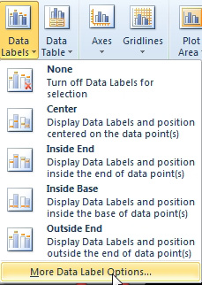
Excel charts: add title, customize chart axis, legend and data labels For example, this is how we can add labels to one of the data series in our Excel chart: For specific chart types, such as pie chart, you can also choose the labels location. For this, click the arrow next to Data Labels, and choose the option you want. To show data labels inside text bubbles, click Data Callout. Add label to Excel chart line • AuditExcel.co.za MS Excel Training Adding a label to an Excel line chart is very easy. As shown below, you can create the chart and then right click on the line and choose 'Add Data Labels' and then 'Add Data Labels' again. The labels are immediately put on the chart and Excel has 'guessed' that you wanted the values to appear. Add a DATA LABEL to ONE POINT on a chart in Excel Click on the chart line to add the data point to. All the data points will be highlighted. Click again on the single point that you want to add a data label to. Right-click and select ' Add data label ' This is the key step! Right-click again on the data point itself (not the label) and select ' Format data label '.
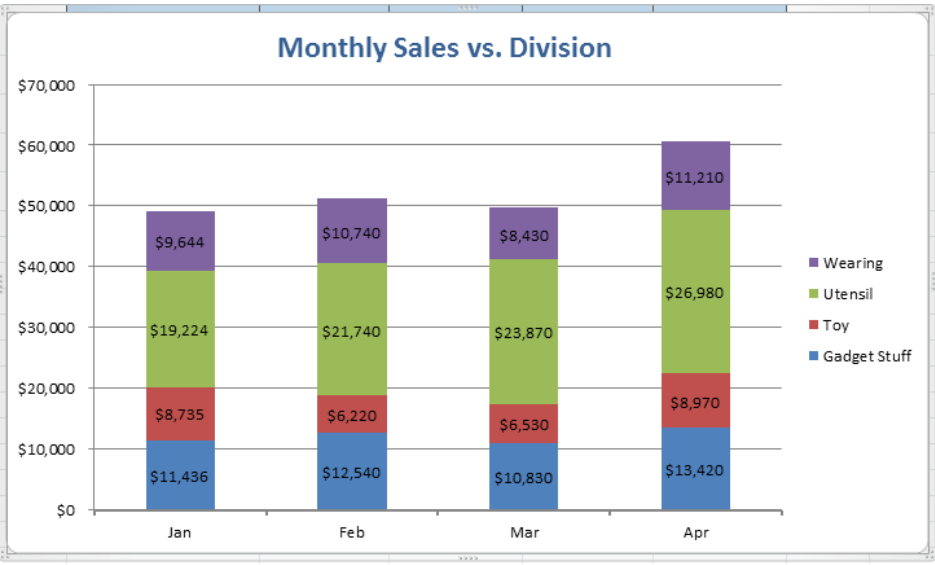
How do i add labels to a chart in excel. how to add data labels into Excel graphs - storytelling with data You can download the corresponding Excel file to follow along with these steps: Right-click on a point and choose Add Data Label. You can choose any point to add a label—I'm strategically choosing the endpoint because that's where a label would best align with my design. Excel defaults to labeling the numeric value, as shown below. How to Add Data Labels to an Excel 2010 Chart - dummies Excel provides several options for the placement and formatting of data labels. Use the following steps to add data labels to series in a chart: Click anywhere on the chart that you want to modify. On the Chart Tools Layout tab, click the Data Labels button in the Labels group. A menu of data label placement options appears: Add Custom Labels to x-y Scatter plot in Excel Step 1: Select the Data, INSERT -> Recommended Charts -> Scatter chart (3 rd chart will be scatter chart) Let the plotted scatter chart be. Step 2: Click the + symbol and add data labels by clicking it as shown below. Step 3: Now we need to add the flavor names to the label. Now right click on the label and click format data labels. How to Add Total Values to Stacked Bar Chart in Excel Step 4: Add Total Values. Next, right click on the yellow line and click Add Data Labels. Next, double click on any of the labels. In the new panel that appears, check the button next to Above for the Label Position: Next, double click on the yellow line in the chart. In the new panel that appears, check the button next to No line:
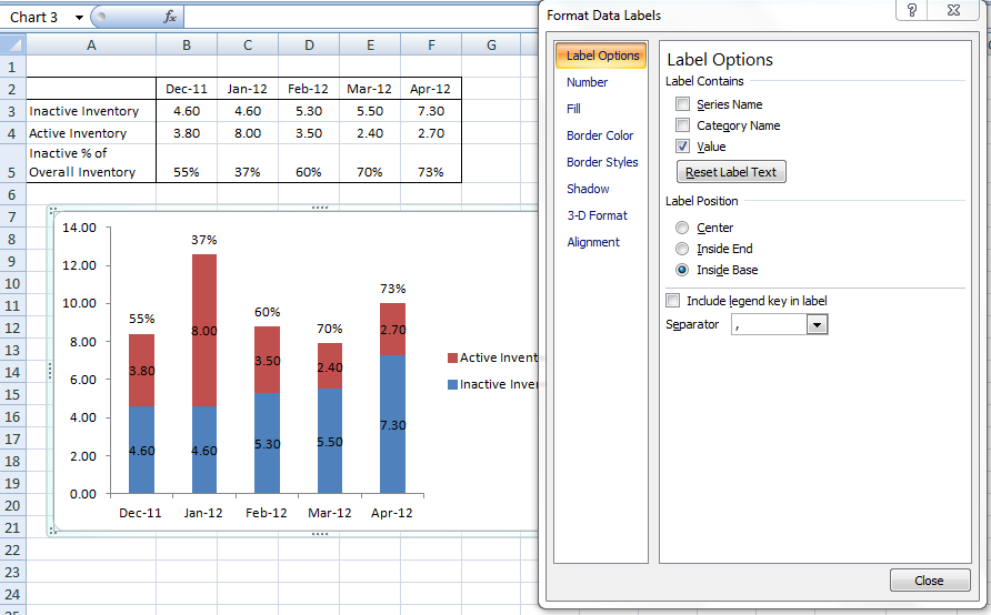
Adding Data Labels to Your Chart (Microsoft Excel) To add data labels, follow these steps: Activate the chart by clicking on it, if necessary. Choose Chart Options from the Chart menu. Excel displays the Chart Options dialog box. Make sure the Data Labels tab is selected. (See Figure 1.) The left side of the dialog box shows the different types of data labels you can choose. How to Place Labels Directly Through Your Line Graph in Microsoft Excel Click on Add Data Labels. Your unformatted labels will appear to the right of each data point: Click just once on any of those data labels. You'll see little squares around each data point. Then, right-click on any of those data labels. You'll see a pop-up menu. Select Format Data Labels. How To Create Labels In Excel — Colleged Enter field names for each column on the first row. Set up labels in word. To import the data, click select recipients > use existing list. Click Inside The Chart Area To Display The Chart Tools. If needed, add an empty row and column between the cards and, optionally, tick off add header and preserve formatting. Address envelopes from lists in ... Labels - How to add labels | Excel E-Maps Tutorial You can add a label to a point by selecting a column in the LabelColumn menu. Here you can see an example of the placed labels. If you would like different colors on different points you should create a thematic layer. You can do this by following the tutorial about Thematic Points and to chooce Individual Colors. You can find the tutorial here.
Edit titles or data labels in a chart - support.microsoft.com On a chart, click the label that you want to link to a corresponding worksheet cell. On the worksheet, click in the formula bar, and then type an equal sign (=). Select the worksheet cell that contains the data or text that you want to display in your chart. You can also type the reference to the worksheet cell in the formula bar. How to Create a Bar Chart With Labels Inside Bars in Excel 7. In the chart, right-click the Series "# Footballers" Data Labels and then, on the short-cut menu, click Format Data Labels. 8. In the Format Data Labels pane, under Label Options selected, set the Label Position to Inside End. 9. Next, in the chart, select the Series 2 Data Labels and then set the Label Position to Inside Base. How to Add Labels to Scatterplot Points in Excel - Statology Step 3: Add Labels to Points. Next, click anywhere on the chart until a green plus (+) sign appears in the top right corner. Then click Data Labels, then click More Options…. In the Format Data Labels window that appears on the right of the screen, uncheck the box next to Y Value and check the box next to Value From Cells. How to Add Data Labels in Excel - Excelchat | Excelchat After inserting a chart in Excel 2010 and earlier versions we need to do the followings to add data labels to the chart; Click inside the chart area to display the Chart Tools. Figure 2. Chart Tools Click on Layout tab of the Chart Tools. In Labels group, click on Data Labels and select the position to add labels to the chart. Figure 3.
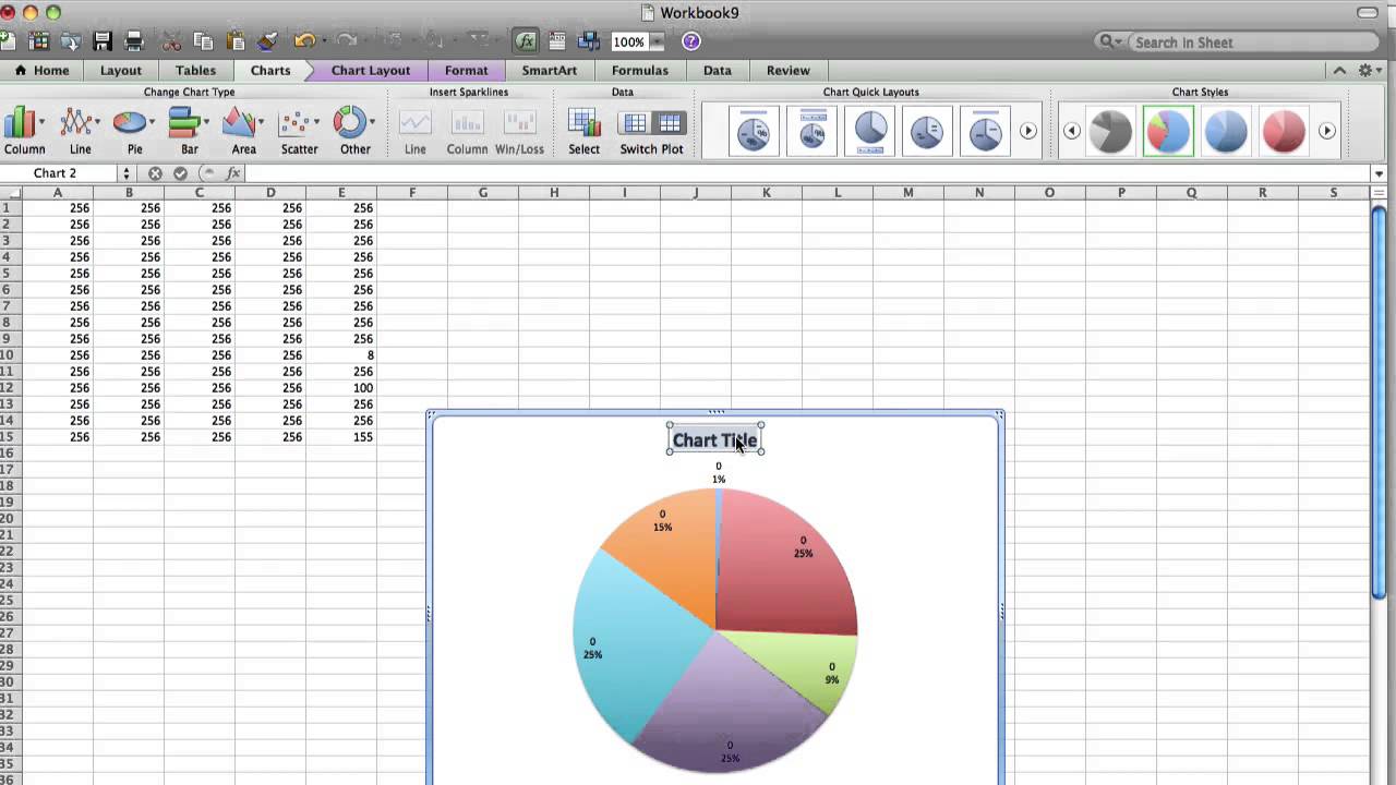
Excel 3-D Pie charts - Microsoft Excel 2010
How to Add Target Line to Pivot Chart in Excel (2 Effective Methods) 2. Using Excel Pivot Table Analyze Tab to Add Pivot Chart Target Line. Another way to add a target line in the Pivot Chart is to use the PivotTable Analyze Tab. You just need to add a new field for this aspect. Let's go through the following description to get a detailed view of this scenario. Steps:

Create a Timeline with Milestones - YouTube
Add or remove data labels in a chart - support.microsoft.com Add data labels to a chart Click the data series or chart. To label one data point, after clicking the series, click that data point. In the upper right corner, next to the chart, click Add Chart Element > Data Labels. To change the location, click the arrow, and choose an option.
Excel Charts: Polar Plot Chart. Polar Plot Created Using Radar Chart
How to Add Axis Labels in Excel Charts - Step-by-Step (2022) How to add axis titles 1. Left-click the Excel chart. 2. Click the plus button in the upper right corner of the chart. 3. Click Axis Titles to put a checkmark in the axis title checkbox. This will display axis titles. 4. Click the added axis title text box to write your axis label.

10 Tips for Making Charts in Excel | Mekko Graphics
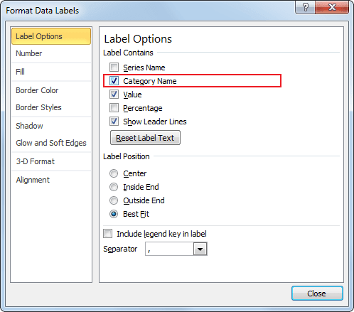
How do you add data labels to a chart in Excel 2016? To format data labels, select your chart, and then in the Chart Design tab, click Add Chart Element > Data Labels > More Data Label Options. Click Label Options and under Label Contains, pick the options you want. To make data labels easier to read, you can move them inside the data points or even outside of the chart.

How to Add Data Labels in Excel - Excelchat | Excelchat
How to add or move data labels in Excel chart? - ExtendOffice To add or move data labels in a chart, you can do as below steps: In Excel 2013 or 2016. 1. Click the chart to show the Chart Elements button .. 2. Then click the Chart Elements, and check Data Labels, then you can click the arrow to choose an option about the data labels in the sub menu.See screenshot:
How to Change Excel Chart Name - YouTube
How to Use Cell Values for Excel Chart Labels Select the chart, choose the "Chart Elements" option, click the "Data Labels" arrow, and then "More Options." Uncheck the "Value" box and check the "Value From Cells" box. Select cells C2:C6 to use for the data label range and then click the "OK" button. The values from these cells are now used for the chart data labels.
How to Add Data Labels in Excel - Excelchat | Excelchat
How to Insert Axis Labels In An Excel Chart | Excelchat We will go to Chart Design and select Add Chart Element Figure 6 - Insert axis labels in Excel In the drop-down menu, we will click on Axis Titles, and subsequently, select Primary vertical Figure 7 - Edit vertical axis labels in Excel Now, we can enter the name we want for the primary vertical axis label.
Excel: Formatting Charts in Excel 2010 with Layout - Excel Articles
Add data labels and callouts to charts in Excel 365 - EasyTweaks.com Step #1: After generating the chart in Excel, right-click anywhere within the chart and select Add labels . Note that you can also select the very handy option of Adding data Callouts.
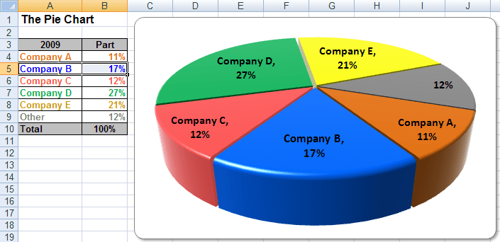
Excel 3-D Pie Charts
How to Add Axis Labels to a Chart in Excel | CustomGuide Select the set of gridlines you want to show. Add Data Labels Use data labels to label the values of individual chart elements. Select the chart. Click the Chart Elements button. Click the Data Labels check box. In the Chart Elements menu, click the Data Labels list arrow to change the position of the data labels. Display a Data Table
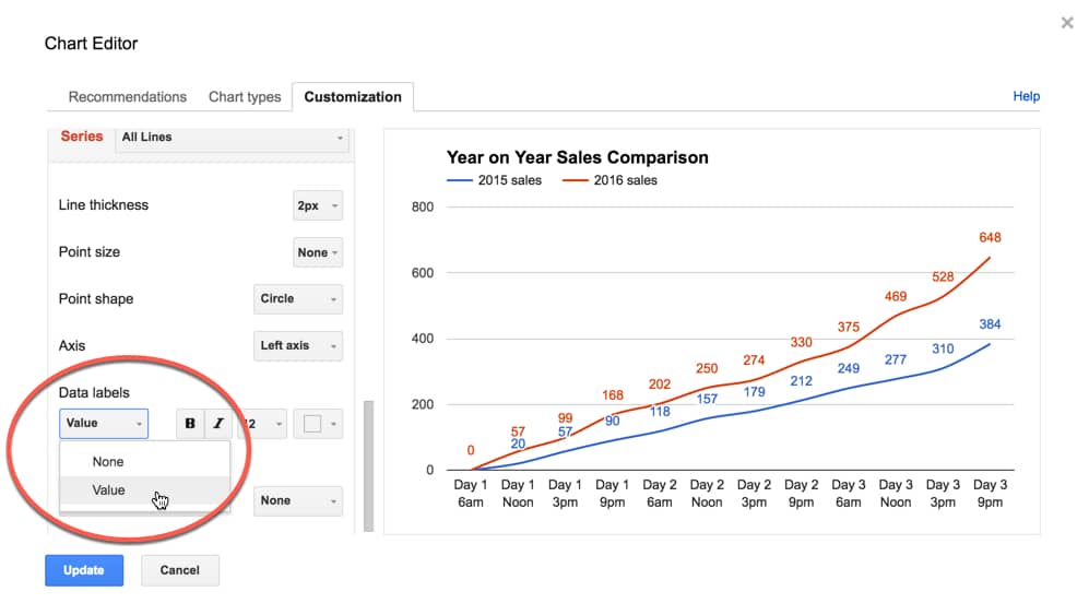
How can I annotate data points in Google Sheets charts? - Ben Collins
Add a DATA LABEL to ONE POINT on a chart in Excel Click on the chart line to add the data point to. All the data points will be highlighted. Click again on the single point that you want to add a data label to. Right-click and select ' Add data label ' This is the key step! Right-click again on the data point itself (not the label) and select ' Format data label '.

Need help making labels on a graph with format code : excel
Add label to Excel chart line • AuditExcel.co.za MS Excel Training Adding a label to an Excel line chart is very easy. As shown below, you can create the chart and then right click on the line and choose 'Add Data Labels' and then 'Add Data Labels' again. The labels are immediately put on the chart and Excel has 'guessed' that you wanted the values to appear.

31 What Is A Label In Excel - Labels For Your Ideas
Excel charts: add title, customize chart axis, legend and data labels For example, this is how we can add labels to one of the data series in our Excel chart: For specific chart types, such as pie chart, you can also choose the labels location. For this, click the arrow next to Data Labels, and choose the option you want. To show data labels inside text bubbles, click Data Callout.

Line Chart in Excel - Easy Excel Tutorial

add labels to excel chart 218253.image0 - Top Label Maker
How-to Put Percentage Labels on Top of a Stacked Column Chart - Excel Dashboard Templates

Excel Chart Elements: Parts of Charts in Excel | ExcelDemy
Post a Comment for "39 how do i add labels to a chart in excel"